The question of identity is a difficult one for microbiologists.
We can usually lump large-bodied organisms together into ecologically and evolutionarily meaningful groups based on distinguishing morphological features (e.g. limbs, eyes, or teeth). Microbes, despite their vast genetic diversity, have a very limited range of shapes and sizes and are too small to see without specialized equipment. Most of them cannot even be grown in the lab. Most confusingly, microorganisms can exchange DNA, making it difficult to trace their genealogy.
Only in the past decade has DNA sequencing technology allowed us to peer into the microbial “dark matter” that permeates our world — the species that were invisible to other laboratory techniques. We’ve come to realize how integral microbial communities are in maintaining the health of the planet and of our bodies. In this protocol, I go over how we identify different microbial groups, or ‘Operational Taxonomic Units’ (OTUs), using molecular sequence data.
Quantifying Diversity
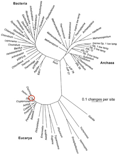
Carl Woese, the father of modern microbial ecology, pioneered the use of the RNA component of the small ribosomal subunit (i.e. known as ‘16S’ in bacteria and archaea and ‘18S’ in eukaryotes) as a molecular fingerprint for distinguishing between all living things. The 16S rRNA gene is required for protein synthesis — a process that is absolutely necessary for staying alive — and is passed from parent to offspring (i.e. no jumping around willy-nilly across the tree of life). The 16S gene has conserved regions that evolve incredibly slowly (i.e. mutations at these sites almost always kill) and variable regions that change more rapidly (i.e. mutations at these sites are less disastrous). The conserved regions conveniently act as anchors that allow for the alignment of sequences from distantly related organisms, while the variable regions can be used to distinguish between more closely related taxa. In this way, Woese built the first comprehensive tree of life, which stretches back almost 4 billion years. Subsequently, the 16S gene has been the workhorse of microbial ecology.
The Wet Lab—DNA extraction and amplification
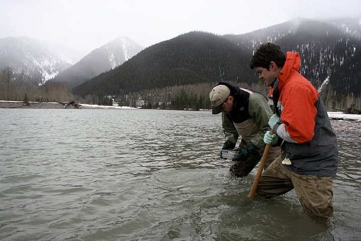
[1.] The first step toward characterizing a microbial community is to collect a sample from an ecosystem where microbes reside, which is to say almost anywhere (e.g. soil, water, poop, air, etc.). Samples are placed in a sterile container and preserved at low temperature or immersed in a chemical cocktail to prevent degradation during the trip back to the laboratory.
[2.] Back in the lab, the samples are liquefied, scraped, and jostled to separate the microbes from the surfaces they are attached to. The resulting cell-slurry is then treated with harsh detergents, heat, and/or mechanical forces (e.g. shaking with silica beads) to burst the cells open and liberate their biomolecular guts (e.g. DNA, RNA, and proteins). Next, the genomic DNA (gDNA) is separated from this molecular soup and purified in a process described in a prior Protocol.
[3.] This purified gDNA blend contains the genomes of all the microbes that once lived in the sample. The next step is to extract the 16S genes. This is done using Polymerase Chain Reaction (PCR), which is a standard process that can produce many billions of copies of a gene from a DNA template. A further purification step removes the original gDNA and we are left with a sample containing a diverse population of short 16S gene fragments. The number of copies of each individual 16S gene is roughly proportional to the abundance of the microbe associated with that gene in the original sample. Details about sample preparation and PCR can be found here.
[4.] PCR products from different samples are labeled with DNA barcodes (short synthetic sequences used to match DNA fragments to samples) and then pooled together and sent to a sequencing facility for processing. There are several high-throughput sequencing technologies available today. Will Trimble, a scientist at Argonne National Laboratory, made this wonderful video that explains one of these technologies.
The Dry Lab—Bioinformatics
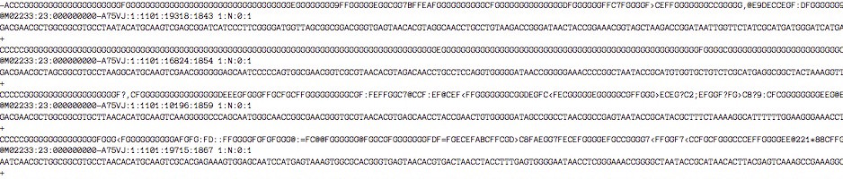
[5.] Once the sequences are ready, the first step is to sort and trim the raw data. Each sequence is referred to as a ‘read.’ Within a read, each DNA base (A, T, C, or G) has a quality score that indicates how confident the sequencer was in making that base call. Low-confidence regions — typically on the ends of reads — are trimmed, and reads with low average confidence scores are discarded. Barcode sequences are used to sort out which sample each read came from. Additional quality control steps can also be run to remove certain PCR and sequencing artifacts. A more comprehensive explanation of Illumina data processing can be found here.

[6.] After quality filtering, the reads are ready to be clustered based on their similarity. Individual sequences are grouped into Operational Taxonomic Units. The most common practice is to bin sequences together at 97% sequence similarity (97% OTUs are thought to approximate ‘species’ in bacteria). This binning can be done by comparing reads to a reference database (i.e. ‘closed reference’ clustering) and matching OTUs to previously sequenced species, clustering reads amongst themselves (i.e. ‘de novo’ clustering), or a hybrid of both reference and de novo clustering (i.e. ‘open reference’ clustering).
However, percent cutoffs are rather arbitrary and are points of serious contention among microbiologists. One obvious flaw in using global cutoffs is that rates of evolution and speciation are not uniform throughout the tree of life. Some researchers argue for more complicated OTU picking methods that infer evolutionary rates to adjust the similarity cutoffs for different lineages. However, these methods are too computationally expensive for very large data sets. The current best practice method is ‘subsampled open reference clustering,’ which uses open reference clustering and can scale to very large data sets.
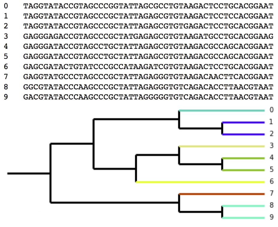
Clustering: Ten sequences clustered at 96% similarity Colors on the branches denote OTUs (seven OTUs total, three with two sequence representatives and four composed of a single sequence).
[7.] After OTU clustering, the number of sequences grouped into each OTU can be tallied across samples. These data are recorded in an n x m matrix with n OTUs and m samples. This is how we go from a soup of molecules to a list of microbial entities whose relative abundances can be tracked across time and space.
Conclusion
Microorganisms are the ancient forbears of life on Earth and are responsible for everything from driving global biogeochemical cycles to maintaining the health and wellbeing of multicellular organisms like us. Knowledge of the structure and function of microbial communities is crucial for our understanding of the biosphere. The protocol described above is referred to as ‘16S amplicon sequencing.’ It is the highest throughput method currently available for studying the composition of microbial ecosystems.